OpenAI published Contrastive Learning Image Pretraining, or CLIP for short on January 5, 2021, alongside DALL-E. Both algorithms were state-of-the-art multimodal algorithms as CLIP could describe text from images and DALL-E could create images from text.
Our focus today will be on implementing a version of CLIP from scratch, with some explanations that can hopefully be helpful. A lot of the work in this article is derived from Matt Nguyen’s work as I took inspiration from his Building CLIP From Scratch article, including the code he used in a Google Colab Implementation. It will be helpful for the purposes of this article if one has a background understanding of encoders, which is a part of the ViT implementation linked below.
Building a Vision Transformer Model From Scratch
We can begin by analyzing the algorithm, and then move on to two different implementations, one that simplifies things, and one that then builds on top of it.
Learning Transferable Visual Models From Natural Language Supervision
The Pseudocode of the original CLIP implementation is available at the link above on page 5, the explanation for which is provided below.
The following steps can be outlined to describe what is happening in CLIP at a high level:
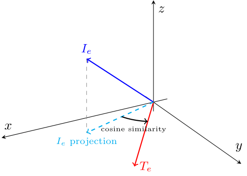
This diagram shows a simplified example in three dimensions, where the Image Embedding is captured in a 3-dimensional vector and the Text Embedding is captured in a 2D vector that lies on the xy plane. In order to get a cosine similarity between the two embeddings, we must first project the Image embedding on to the xy plane. We can then calculate the cosine similarity between the two vectors. In reality however, the dimensionality is much higher than this, so this is only an easy way to visualise the process. With CLIP, the goal is to determine how well an image matches a given text description, and this can be done by calculating the cosine similarity between their embeddings.
Now that we have an understanding of how CLIP works, we can implement it. However, it has already been implemented from scratch before, so I wanted to experiment with things a bit. In the original Google Colab notebook by Matt Nguyen, he used a Vision Transformer built from scratch to obtain the image encodings, and a transformer (tokenizer too) that he built to get the text encodings. What if we replaced these transformers to use different pre-trained options? How well would this work for something like the FashionMNIST dataset if we use pre-trained encoders?
The Google Colab notebook for this part can be found here.
After importing the libraries,
import torch
import torch.nn as nn
import torch.optim as optim
import torchvision.transforms as T
from torch.utils.data import Dataset, DataLoader
from datasets import load_dataset
import matplotlib.pyplot as plt
import numpy as np
we can choose a text encoder. We can use BERT as it is a famous model built with transformers, and the tokenizer model should be useful for our purposes. We have to make sure that we freeze the parameters for this model, as the goal is to find out how well it works off the shelf. The projection to the embedding dimension should, however, still be trainable.
from transformers import BertTokenizer, BertModel

class TextEncoder(nn.Module):
    def __init__(self, emb_dim):
        super().__init__()

        # Using a pre-trained BERT model
        self.bert = BertModel.from_pretrained('bert-base-uncased')
        for param in self.bert.parameters():
            param.requires_grad = False  # Freeze BERT parameters

        # Adding a linear projection to get to the embedding dimension
        self.projection = nn.Linear(self.bert.config.hidden_size, emb_dim)

    def forward(self, text):
        # Tokenizing text before passing it in, also not training this
        with torch.no_grad():
            outputs = self.bert(**text)
            x = outputs.last_hidden_state[:, 0, :]

        # Projecting to wanted dimension
        x = self.projection(x) # Trainable Projection
        x = x / torch.norm(x, dim=-1, keepdim=True)  # L2 normalization

        return x
Similarly, we can replace the Image Encoder with a CNN-based network. I chose ResNet50 for the purpose of this tutorial, as I expected it to run faster in comparison to ViT. I was also curious as to how well a CNN embedding would perform for the overall model. We are also freezing parameters and projecting to an embedding dimension here. We have to remember to remove the final classification layer, as the goal is to simply pass the embedding information along. The final output layer has an output dimension of 2048, before the classification layer.
from torchvision import models
import torch.nn.functional as F

class ImageEncoder(nn.Module):
    def __init__(self, emb_dim):
        super().__init__()

        # Using a pre-trained ResNet for image embeddings
        self.resnet = models.resnet50(weights='IMAGENET1K_V1')
        for param in self.resnet.parameters():
            param.requires_grad = False  # Freeze ResNet parameters

        # Removing the final classification layer
        self.resnet = nn.Sequential(*list(self.resnet.children())[:-1])

        # Final output layer dimension
        self.output_dim = 2048

        # Adding a linear projection to get to the embedding dimension
        self.projection = nn.Linear(self.output_dim, emb_dim)

    def forward(self, x):
        # Extracting image features using ResNet, but not training
        with torch.no_grad():
            x = self.resnet(x)  # Shape: (batch_size, 2048, 1, 1)
        x = x.view(x.size(0), -1) # Flatteing output to: (batch_size, 2048)

        # Projecting to wanted dimension
        x = self.projection(x)  # Shape: (batch_size, emb_dim)
        x = F.normalize(x, p=2, dim=-1)  # L2 normalization

        return x
We can then set up the CLIP algorithm where we get image and text embeddings, and then we can calculate the scaled pairwise cosine similarities between every image-text pair in the batch. After that, we calculate the loss function. The latter parts of the function including the cosine similarities calculation and loss function calculation are the same as the Building CLIP From Scratch tutorial.
class CLIP(nn.Module):
    def __init__(self, emb_dim):
        super().__init__()

        # Use the previously created encoders
        self.image_encoder = ImageEncoder(emb_dim)
        self.text_encoder = TextEncoder(emb_dim)

        # Temperature parameter for scaling cosine similarity
        self.temperature = nn.Parameter(torch.ones([]) * np.log(1 / 0.07))
        self.device = torch.device("cuda" if torch.cuda.is_available() else "cpu")

    def forward(self, image, text):
        I_e = self.image_encoder(image)
        T_e = self.text_encoder(text)

        # cosine similarities
        logits = (I_e @ T_e.transpose(-2, -1)) * torch.exp(self.temperature)

        # loss function
        labels = torch.arange(logits.shape[0]).to(self.device)
        loss_i = nn.functional.cross_entropy(logits.transpose(-2, -1), labels)
        loss_t = nn.functional.cross_entropy(logits, labels)
        loss = (loss_i + loss_t) / 2

        return loss
For the next portion, we need to create a class for the Dataset. We need to pre-process the dataset so that we can return valid information that is useful to the ResNet50 and BERT models. FashionMNIST doesn’t come with generated captions, instead it comes with labels for each class. We simply have to add some captions to each class. We also make each image “RGB” by simply repeating the image 3 times, as that is the format ResNet50 expects.
class FashionMNIST(Dataset):
    def __init__(self, train=True):
        self.dataset = load_dataset("fashion_mnist")
        self.transform = T.ToTensor() # need this for ResNet
        self.tokenizer = BertTokenizer.from_pretrained('bert-base-uncased')

        # This is for future splitting of the dataset
        self.split = "train" if train else "test"

        # Creating captions to map the labels to
        self.captions = {
            0: "An image of a t-shirt/top",
            1: "An image of trousers",
            2: "An image of a pullover",
            3: "An image of a dress",
            4: "An image of a coat",
            5: "An image of a sandal",
            6: "An image of a shirt",
            7: "An image of a sneaker",
            8: "An image of a bag",
            9: "An image of an ankle boot"
        }

    def __len__(self):
        return self.dataset.num_rows[self.split]

    def __getitem__(self, i):
        img = self.dataset[self.split][i]["image"]
        img = self.transform(img)

        # Converting 1-channel grayscale image to 3-channel RGB
        img = img.repeat(3, 1, 1)

        # matching caption to label
        label = self.dataset[self.split][i]["label"]
        caption = self.captions[label]

        # Tokenizing the caption
        # The tokenizer usually returns an extra dimension
        #    so we remove that with squeeze(0)
        encoded_caption = self.tokenizer(caption, return_tensors='pt', padding='max_length', truncation=True, max_length=32)
        input_ids = encoded_caption['input_ids'].squeeze(0)
        attention_mask = encoded_caption['attention_mask'].squeeze(0)

        # returning everything as flat tensors, this could effect performance
        return img, input_ids, attention_mask, label
We can then set up the hyperparameters and load the dataset for usage in training.
emb_dim = 512
lr = 1e-4
epochs = 10
batch_size = 64

train_set = FashionMNIST(train = True)
test_set = FashionMNIST(train = False)

train_loader = DataLoader(train_set, shuffle=True, batch_size=batch_size)
test_loader = DataLoader(test_set, shuffle=False, batch_size=batch_size)
The training loop is in the code block below. We initialize the CLIP model with the embedding dimension that want and set up the optimizer. Since we want to see how the model performs using off-the-shelf embeddings, we have to set up which parameters will be optimized. We only want to optimize the embedding projections and the temperature. The loop then iterates over epochs, where the model computes the loss by comparing the cosine similarities between the text and image embeddings. We then perform backpropagation where the gradients are calculated and the model’s parameters are updated to minimize the loss. The best model is saved at the end of each epoch. I also added a timer in order to get a sense of training time.
device = torch.device("cuda" if torch.cuda.is_available() else "cpu")
print("Using device: ", device, f"({torch.cuda.get_device_name(device)})" if torch.cuda.is_available() else "")

# Initializing CLIP
model = CLIP(emb_dim).to(device)

# Optimizer setup
# Collect parameters to optimize
params = list(model.image_encoder.projection.parameters()) + \
         list(model.text_encoder.projection.parameters()) + \
         [model.temperature]

optimizer = optim.Adam(params, lr=lr)

best_loss = np.inf
for epoch in range(epochs):
    start_time = time.time()
    model.train()  # Set model to training mode

    for batch in train_loader:
        # unpacking the whole batch for training
        images = batch[0].to(device)
        input_ids = batch[1].to(device)
        attention_mask = batch[2].to(device)

        text_inputs = {"input_ids": input_ids, "attention_mask": attention_mask}
        loss = model(images, text_inputs)

        # Backpropagation and optimization
        optimizer.zero_grad()
        loss.backward()
        optimizer.step()

    # Logging the loss
    print(f"Epoch [{epoch + 1}/{epochs}], Loss: {loss.item():.4f}")

    # Save the best model
    if loss.item() < best_loss:
        best_loss = loss.item()
        torch.save(model.state_dict(), "clip_model.pt")
        print("Model Saved.")

    end_time = time.time()
    print(f"Time taken for epoch {epoch + 1}: {end_time - start_time:.2f} seconds")
Next, we set up the evaluation loop, starting by loading the trained model and setting it to evaluation mode. We begin by precomputing the text embeddings for the class descriptions, as these embeddings remain fixed throughout the testing process.
For each batch in the test dataset, we extract the images and their corresponding true labels. We then generate image embeddings using the image encoder and calculate the cosine similarity between these embeddings and the pre-computed text embeddings. This similarity score quantifies how well the image aligns with each class description. The predicted label is determined by identifying the class with the highest similarity score.
Finally, we compare the predicted labels to the true labels, tallying the correct predictions to compute the overall test accuracy.
# Loading saved model and setting up for evaluation
model = CLIP(emb_dim).to(device)
model.load_state_dict(torch.load("clip_model.pt"))
model.eval()

# computing the embeddings for the class labels
class_names = ["An image of a t-shirt or top", "An image of trousers", "An image of a pullover", "An image of a dress", "An image of a coat",
               "An image of sandals", "An image of a shirt", "An image of sneakers", "An image of a bag", "An image of ankle boots"]

# tokenizing the above labels
text_inputs = test_set.tokenizer(class_names, padding=True, truncation=True, return_tensors="pt").to(device)
# no_grad() here maybe unnecessary, the goal is to not train anything when pre-computing embeddings
with torch.no_grad():
    class_text_features = model.text_encoder(text_inputs)

correct, total = 0, 0

for batch in test_loader:
    images = batch[0].to(device)
    labels = batch[3].to(device)

    with torch.no_grad():
        image_features = model.image_encoder(images)

    # calculate similarities
    similarities = image_features @ class_text_features.T

    # predicted labels are the indices of the maximum similarity scores
    preds = similarities.argmax(dim=1)

    # update accuracy
    correct += (preds == labels).sum().item()
    total += labels.size(0)

print(f"Test Accuracy: {correct / total:.4f}")
For the last step, we demonstrate the zero-shot classification capabilities of CLIP. Similar to the above, we load the saved model, pre-compute the text embeddings, and generate the image embeddings for a single image that we have not trained on. We calculate the cosine similarity, which allows the model to rank the classes, and finally, we display the top 5 predicted class names, along with their associated probabilities.
# loading saved model
model = CLIP(emb_dim).to(device)
model.load_state_dict(torch.load("clip_model.pt"))
model.eval()

class_names = ["An image of a t-shirt or top", "An image of trousers", "An image of a pullover", "An image of a dress", "An image of a coat",
               "An image of sandals", "An image of a shirt", "An image of sneakers", "An image of a bag", "An image of ankle boots"]

# pre-computing text embeddings
text_inputs = test_set.tokenizer(class_names, padding=True, truncation=True, return_tensors="pt").to(device)
with torch.no_grad():
    text_features = model.text_encoder(text_inputs)

# get image embeddings for image and then plot image
idx = 2000
img, _, _, label = test_set[idx]  # Unpack image and label
img_cpu = img.cpu()
plt.imshow(img_cpu.permute(1, 2, 0).squeeze(), cmap="gray")
plt.title(class_names[label])
plt.show()

img_tensor = img.unsqueeze(0).to(device)
with torch.no_grad():
    # using model to calculate similarity
    image_features = model.image_encoder(img_tensor)
    similarity = (image_features @ text_features.T).softmax(dim=-1)
    values, indices = similarity[0].topk(5)

# printing result
print("\nTop predictions:\n")
for value, index in zip(values, indices):
    print(f"{class_names[int(index)]:>30s}: {100 * value.item():.2f}%")
The question I attempted to answer in the above section is, ‘Can pre-trained models immediately replace the encoders in a CLIP implementation?’
The test accuracy I obtained was 75.65%, whereas the test accuracy for the implementation from scratch was 84% (hyper-parameter tuning can certainly improve performance even further.) Considering that we do not perform any further training for ResNet or BERT on this dataset, I am quite impressed with the performance.
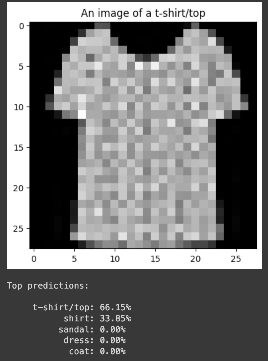
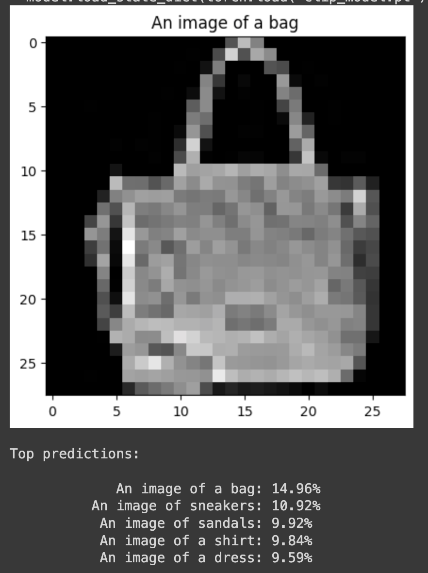
One of my major points of concern, however, is that while the model is still correct around 76% of the time, the spread of probability over all the classes is a weakness. The original model was consistently more confident in the correct answer. This can be attributed to the fact that we did not fine-tune ResNet and BERT. It could also be because of the alignment differences in between ResNet and BERT. They both generate embeddings that work within their own contexts, but when they are used for dimensions specific to FashionMNIST, there might be less coherence in between the two.
While setting up the functions in the previous notebook to have trainable layers for BERT and ResNet, I was curious about working with a different dataset. The datasets library is a great resource for finding something suitable. Since both BERT and ResNet were trained on diverse datasets, I wanted to check the capabilities of this local CLIP model if we also got a diverse dataset.
While I initially started with a fork of the COCO dataset containing image URLs and 5 sentences describing each image, the training time was too high because each image had to be downloaded. I decided to then move on to the Flickr8k dataset linked below, as the images came included and I only wanted to experiment with one caption per image (even though it has two more synthetically created.)
kargwalaryan/SynCap-Flickr8k · Datasets at Hugging Face
You can follow along with my implementation here.
We should not have to change too much in order to adapt the code to a new dataset.
The library imports should remain the same, but we do need to change a few lines for the text encoder portion. We now open up the last three layers of BERT for training and the torch.nograd() portion is removed.
from transformers import BertTokenizer, BertModel

class TextEncoder(nn.Module):
    def __init__(self, emb_dim):
        super().__init__()

        self.bert = BertModel.from_pretrained('bert-base-uncased')

        # the last three layers of the network are open for training
        for name, param in self.bert.named_parameters():
            if 'encoder.layer.11' in name or 'encoder.layer.10' in name or 'pooler' in name:
                param.requires_grad = True
            else:
                param.requires_grad = False

        self.projection = nn.Linear(self.bert.config.hidden_size, emb_dim)

    def forward(self, text):
        outputs = self.bert(**text)
        x = outputs.last_hidden_state[:, 0, :]

        x = self.projection(x)
        x = x / torch.norm(x, dim=-1, keepdim=True)

        return x
Similarly, we open up the last layer of ResNet for training in the ‘ImageEncoder’ block.
for name, param in self.resnet.named_parameters():
            if 'layer4' in name:
                param.requires_grad = True
            else:
                param.requires_grad = False
The major change comes in the form of the dataset class. We can load the dataset but since all of it falls under the “train” split, we need to manually create a split ourselves. We also need to resize the images to 224 by 224 pixels and normalize them (based on ImageNet) as that is what is expected by ResNet in our Image Encoder class. We then extracted the caption and tokenized it using the BertTokenizer similar to the previous notebook.
class Flickr8kDataset(Dataset):
    def __init__(self, train=True):
        # loading dataset and splitting it
        dataset = load_dataset("kargwalaryan/SynCap-Flickr8k")
        split_dataset = dataset["train"].train_test_split(test_size=0.2, seed=42)
        self.tokenizer = BertTokenizer.from_pretrained('bert-base-uncased')
        # resize the images, make it a tensor, then normalise it
        self.transform = T.Compose([
            T.Resize((224, 224)),
            T.ToTensor(),
            T.Normalize(mean=[0.485, 0.456, 0.406], std=[0.229, 0.224, 0.225])
        ])
        # Simple way to return split
        if train:
            self.dataset = split_dataset['train']
        else:
            self.dataset = split_dataset['test']

    def __len__(self):
        return len(self.dataset)

    def __getitem__(self, idx):
        # get the image and then convert it to remove any grayscale images
        # This is a more elegant method than repeating it thrice
        img = self.dataset[idx]['image']
        img = img.convert("RGB")
        img = self.transform(img)
        # get the caption then tokenize it
        caption = self.dataset[idx]['caption']
        encoded_caption = self.tokenizer(caption, return_tensors='pt', padding='max_length',
                                         truncation=True, max_length=32)
        # Getting the numerical ID's of the tokens and the attention mask
        input_ids = encoded_caption['input_ids'].squeeze(0)
        attention_mask = encoded_caption['attention_mask'].squeeze(0)
        return img, input_ids, attention_mask
We set up the training parameters and load the dataset like before, the main change occurs in the training loop. We now have to add some options to the optimizer that we used, as we have more parts that we want to change. For this experiment, I left the learning rate for ResNet and BERT lower than hyperparameter ‘lr’, and this can be tuned later to improve performance.
optimizer = optim.Adam([
    {'params': model.image_encoder.resnet.parameters(), 'lr': 1e-5},
    {'params': model.text_encoder.bert.parameters(), 'lr': 1e-5},
    {'params': model.image_encoder.projection.parameters(), 'lr': lr},
    {'params': model.text_encoder.projection.parameters(), 'lr': lr},
    {'params': [model.temperature], 'lr': lr}
])
The testing loop will also be quite different as I focused more on checking the Image to Text retrieval capabilities of the model. We first load the model, then we load all the image and text embeddings. We then connect all embeddings which allows us to create a similarity matrix for all the pairs.
For each image, we extract the corresponding row of the similarity matrix, as this row contains the similarity scores between the image and all the text embeddings. We then sort the similarities in descending order (highest similarity first), and then check for the index of the correct text embedding. We then calculate the rank, which is essentially where in the list the correct caption lies. The higher the rank, the worse it is.
Finally, for some metrics, we calculate recall, which is the percentage of times the correct caption appears within the top N-ranked captions for each image.
# Loading the model and enabling evaluation
model = CLIP(emb_dim).to(device)
model.load_state_dict(torch.load("clip_model.pt"))
model.eval()

# calculating the image and text embeddings for all items in test dataset
image_embeddings = []
text_embeddings = []

with torch.no_grad():
    for batch in val_loader:
        images = batch[0].to(device)
        input_ids = batch[1].to(device)
        attention_mask = batch[2].to(device)
        text_inputs = {"input_ids": input_ids, "attention_mask": attention_mask}

        image_features = model.image_encoder(images)
        text_features = model.text_encoder(text_inputs)

        image_embeddings.append(image_features)
        text_embeddings.append(text_features)

# connecting all embeddings
image_embeddings = torch.cat(image_embeddings, dim=0)
text_embeddings = torch.cat(text_embeddings, dim=0)

# get the similarity for all image-text pairs
similarity_matrix = image_embeddings @ text_embeddings.T

# see how well the model performed in relation to all options
ranks = []
for i in range(len(image_embeddings)):
    sims = similarity_matrix[i]
    sorted_indices = torch.argsort(sims, descending=True)
    rank = (sorted_indices == i).nonzero(as_tuple=True)[0].item() + 1
    ranks.append(rank)

# calculate and display the recall, explained above
ranks = np.array(ranks)
recall_at_1 = np.mean(ranks <= 1) * 100
recall_at_5 = np.mean(ranks <= 5) * 100
recall_at_10 = np.mean(ranks <= 10) * 100

print(f"Image-to-Text Retrieval:")
print(f"Recall@1: {recall_at_1:.2f}%")
print(f"Recall@5: {recall_at_5:.2f}%")
print(f"Recall@10: {recall_at_10:.2f}%")
Instead of doing a zero-shot classification as we are not training on chunks of data, I wanted to visualize the final results and captions that are chosen. We first choose (randomly) the indices for the images we want to work with. Then we get the image embedding for them and calculate the similarity against the text embeddings. We then rank them and the top N captions are displayed alongside the picture.
import matplotlib.pyplot as plt

# how many examples and captions do I want?
num_examples = 5
K = 5

# randomly select indices from the validation dataset
indices = np.random.choice(len(val_dataset), num_examples, replace=False)

# For each image
for idx in indices:
    img, input_ids, attention_mask = val_dataset[idx.item()]
    img_tensor = img.to(device).unsqueeze(0)

    # Get the image embedding and calculate similarity
    with torch.no_grad():
        image_feature = model.image_encoder(img_tensor)
        sims = image_feature @ text_embeddings.T
        sims = sims.squeeze(0)

    # get the top k captions for said image
    topk_indices = torch.argsort(sims, descending=True)[:K]
    topk_indices = [int(i.item()) for i in topk_indices]

    topk_captions = [val_dataset.dataset[i]['caption'] for i in topk_indices]

    # Showing the top k images and their captions
    plt.imshow(img.permute(1, 2, 0).cpu())
    plt.axis('off')
    plt.show()

    print(f"Top {K} Captions for Image Index {idx}:")
    for i, caption in enumerate(topk_captions):
        print(f"{i+1}: {caption}")
    print("\n")
The model did not perform as well as I had expected after FashionMNIST implementation.
While I was immensely disappointed as I expected it to perform better, once I started looking at the possible captions for the images themselves it started to make sense to me.

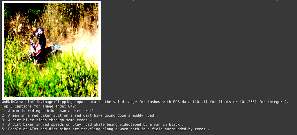
The loss on the training data in the 15 epochs I trained had climbed down to 0.3921 from a starting point of 1.6041, so I expected better results. However, once we see the captions available, I see that there are many similar images with similar captions. So, even though the model is not getting the correct caption immediately, it can definitely focus on the important parts of the image and get near the ballpark of the correct text embedding.
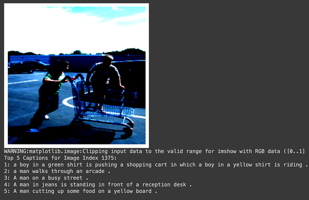
When the caption is correct in the first position, it’s because the image and captions were unique enough to be related. For example, in Figure 3b, the model correctly identifies the image with “A boy in a green shirt is pushing a shopping cart in which a boy in a yellow shirt is riding.” The scenario is so unique that the rest of the options (in the top 5) are not adequate to describe this.
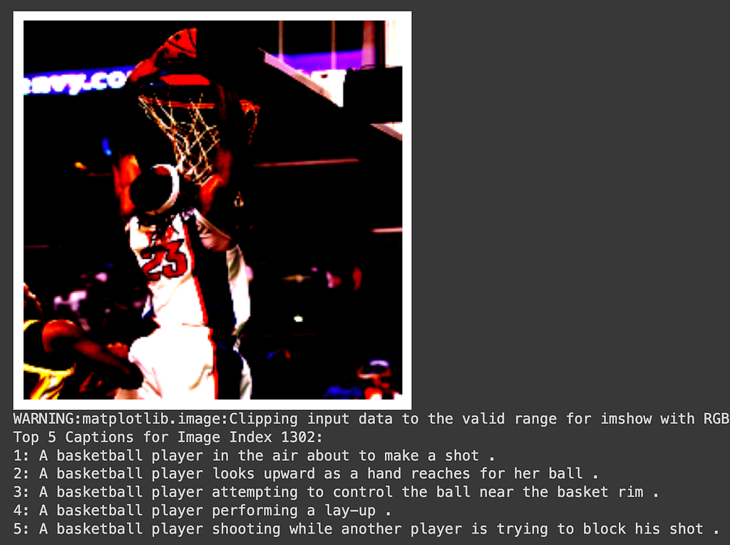
However, when we have many caption options for one image, the model struggles the most. For example, in Figure 5a, there is clearly a basketball player making a slam dunk, but the model is struggling to choose the correct option. The words “a basketball player” are clearly present in all the top 5 options, however, the embedding isn’t differentiated enough to describe it.
I believe that using a ViT for the image encoder may fix some of these issues as the overall context could then be considered. Also, further training (fine tuning) can help lower the loss, but there is a fear of overfitting this new dataset.
<hr><p>CLIP implementation with pre-trained embeddings was originally published in Toward Humanoids on Medium, where people are continuing the conversation by highlighting and responding to this story.</p>