The goal of this article is to analyze the paper “Deep Transformer Q-Networks for Partially Observable Reinforcement Learning” by Kevin Esslinger, Robert Platt, and Christopher Amato while learning some of the background and history along the way.
Deep Transformer Q-Networks for Partially Observable Reinforcement Learning
Let’s first start with a little bit of information regarding reinforcement learning.
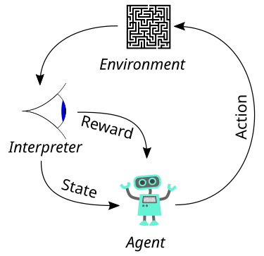
What is RL? It’s a type of machine learning where an agent learns to take the best sequence of actions in an environment to maximize its final reward. This scenario is well captured by the image below.
When modeling this kind of scenario, a good mathematical framework is the Markov Decision Process. The Markov property, states that “future states depend only on the current state and action, not the whole history.” This is important for us, as when the agent takes an action within the environment from some state, it may obtain a reward along the way, but the next state it lands in is only dependent upon the current state and action taken. The medium article by Nan below does an amazing job of explaining Markov Decision Processes with a grid world example.
Markov decision process: basics
Given that you have a perfect model of your environment, meaning your transition function and reward function are accurate enough, we can use exact solution methods to obtain the optimal value for each state. The basic two exact solution methods I started with are Value Iteration and Policy Iteration.
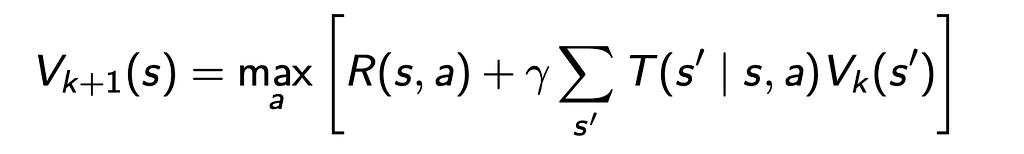
Value iteration involves iteratively updating the utility values for each state using the Bellman Update until we converge on the optimal value function V* for each state.
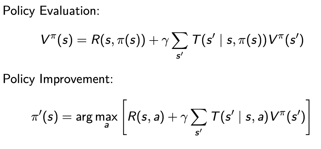
We can also use Policy Iteration, where we iteratively go through two steps, policy evaluation and policy improvement until we converge on the optimal policy for each state. Policy iteration can be more efficient than value iteration in certain cases and it requires fewer iterations to converge.
Two other articles also written by Nan are great resources for obtaining a thorough understanding of Value Iteration and Policy Iteration.
But what happens when we don’t know the transition function or the reward function for the environment?
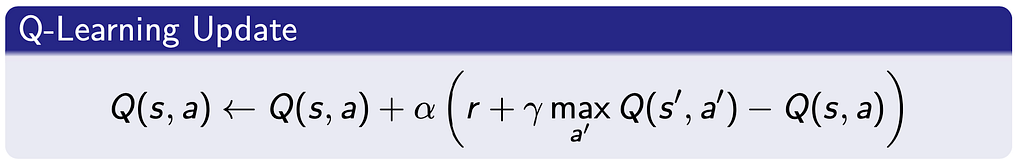
We can’t use exact solution methods anymore, but we can use Model-Free Methods to learn the value function or policy directly by interacting with the environment. One such method is called Q-Learning which learns the Q values (i.e. expected cumulative rewards for taking an action in a state) for each state-action pair. Q-learning achieves this by making a table to store the Q values for all states and all actions, then interacting with the environment for a specified number of episodes (a certain number of steps), and updating the Q value for each state-action pair.
For a deeper understanding of Q-Learning, I have linked an article below that is detailed and helps to visualize the process.
Reinforcement Learning Explained Visually (Part 4): Q Learning, step-by-step
What if we cannot simply model the environment with a discrete state space?
If we require a continuous state space, we cannot get away with storing all the Q-values in a table anymore as we now have a potentially infinite number of states for our agent to interact with.
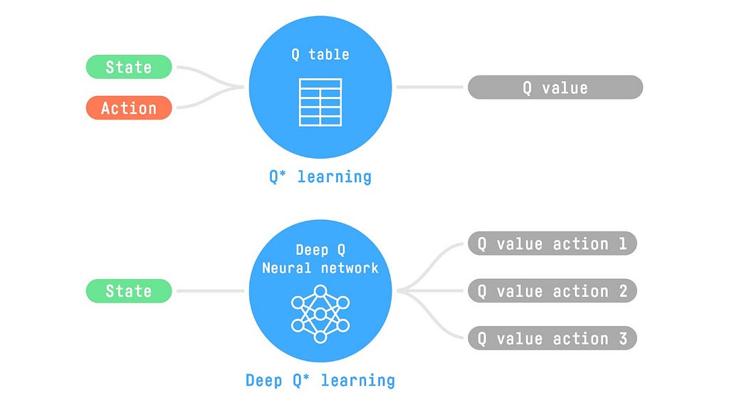
Deepmind came up with a solution for this in 2013 with the paper “Playing Atari with Deep Reinforcement Learning.” They showed that by introducing neural networks to approximate the Q-value function, they could scale to large state spaces.
Playing Atari with Deep Reinforcement Learning
For a deeper understanding of DQN, I highly recommend the articles linked below. They both cover visual explanations of concepts that make DQN perform well, like two Q-networks (a main network and a target network) and an experience replay buffer (we sample random batches from this) which is used to break the correlation between sequential experiences.
What if we don’t know our current state in the environment?
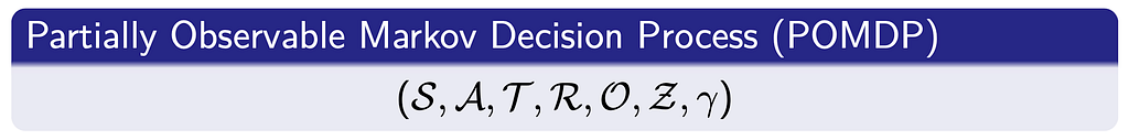
The real world has noisy sensor readings and other uncertainties that make modeling environments using just MDPs difficult. We can then model the environment as a Partially Observable Markov Decision Process. A POMDP now has O, a set of possible observations, and Z, a function that maps to an observation given the next state obtained from an action. Since we do not know the state directly, we can make observations and infer the possible state of the agent by maintaining a belief state.
There already exist techniques to solve POMDPs like QMDP, SARSOP, MCVI, and more. To learn more details regarding POMDPs, please go to the site below.
Deep Recurrent Q Networks
For larger, more complex state spaces in partially observable environments, traditional POMDP solvers often become computationally impractical. Here, Deep Recurrent Q Networks (DRQNs) offer a deep learning-based solution by using recurrent neural networks (like LSTMs) to learn and retain a memory of past observations and actions, helping to approximate the belief state without explicit belief tracking. Long Short-Term Memory (LSTM) networks are used by DRQNs to implicitly learn the underlying state.
Deep Recurrent Q-Learning for Partially Observable MDPs
The page below provides an implementation of a DRQN. Compared to a DQN, the first fully connected layer is replaced by an LSTM layer in DRQN.
If using an RNN (and changing the model) can improve the performance of a DQN, couldn’t transformers improve the performance even further? That is basically what was explored by Esslinger et al. in their paper “Deep Transformer Q-Networks for Partially Observable Reinforcement Learning.”
Transformers are shown to be capable of modeling sequences better than RNNs and the attention mechanism in transformers allows the model to weigh the importance of different parts of the input. Attention is especially helpful in situations like these where we require long-term planning.
For an in-depth understanding of transformers, please refer to the article below, with a particular focus on the decoder portion of the text embedding section.
Architecture
The architecture of a DTQN consists of three main components: Observation Embedding, Transformer Decoder, and Q-Value Head. The input embedding layer encodes the sequence of observations and actions into a suitable format for the transformer. The transformer Decoder then processes these embeddings (leveraging self-attention to model dependencies) and generates an output. We then have a linear transformation to obtain Q-values for each possible action.
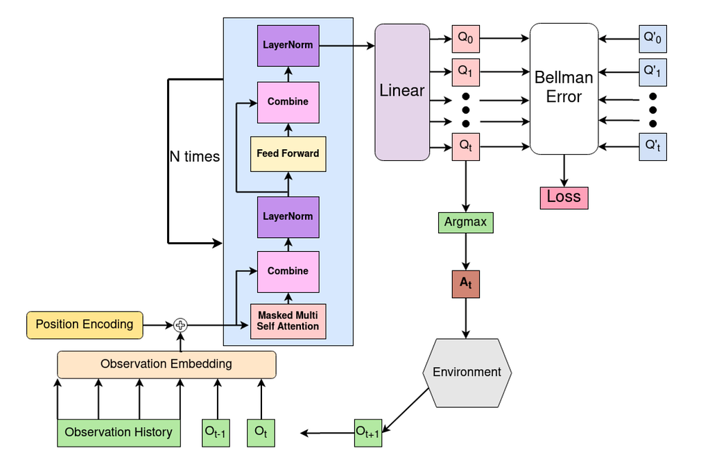
From the image of the architecture above, we can see that we have an input embedding, which takes the current and past observations. There is an optional positional encoding portion that can then be added to this. The embedding is then added to the decoder block, which is a stack of Self-Attention, Combine, LayerNorm, and FeedForward layers. The generated output of the decoder is then fed into the Q-value head (simple linear transformation) and we then obtain the Q-values for each possible action. We calculate loss similar to DQN, take action with the highest Q-value, interact with the environment, and finally add the new observation to the embedding to repeat the whole process over again.
Experiments
The authors compared the performance of DTQN against other networks such as DRQN, DQN, and a basic attention network. They compared performances across several domains such as gym-gridverse, and car flag.
They ran ablation studies to potentially catch which parts of the architecture contributed the most. The base DTQN they used had standard residual connections, where a LayerNorm is applied after the residual connection step. They performed an ablation study by adding gating mechanisms similar to “Gated Recurrent Units” in the “Combine” step in the decoder. They also compared to an Identity map re-ordering variant of the decoder, where LayerNorm occurs before sublayers like “Self-Attention.”
The authors also compared a learned positional encoding versus a sinusoidal positional encoding variant in the study. For the last major comparison, they choose to compare between using the Q-value at the last timestep or the intermediate Q-values at each timestep.
Running DTQN locally
Thankfully, the authors provide a modular set of code that can let us also run DTQN and observe comparisons. The results obtained by the authors can be seen in the original paper where it is well visualized.
I ran some experiments locally with the code available at the repo linked below, and I will include those graphs here alongside instructions on getting set up.
GitHub - kevslinger/DTQN at paper
First of all, please make sure that you clone the “paper” branch of the repo to get the most stable version for replicating the original results.
Given your operating system, some of the instructions on the repo may be outdated, so I’ve included a few extra steps below. If your system cannot make a virtual environment for Python 3.8, you can add older versions with the following command:
sudo add-apt-repository ppa:deadsnakes/ppa
Note, that I used Ubuntu 24.04 to run the experiments, and I did not have Python 3.8 available natively. You can then make a virtual environment following the commands from the repo.
virtualenv venv -p 3.8
source venv/bin/activate
At this point, you should check the version of pip. Quite a few of the requirements listed in the repo are old, and reference requirements with an older style, which can break many installations if you are using a newer version of pip. I downgraded to pip 21.1.3 in order for things to install smoothly.
pip install pip==21.1.3
You can then install all files from the requirements, as mentioned in the repo.
pip install -r requirements.txt
I also recommend installing gym-gridverse, rl-parsers, one-to-one, and gym-pomdps as mentioned in the repo (in that order.)
Results
We can save and visualize the policies obtained from training the agents. The repo suggested using the website wandb.ai, which I would also recommend as it makes it simple to create graphs and have the data in one place. I ran a DQN, DRQN, and DTQN version of the CarFlag environment, each one took ~2 hours to train locally on my GPU.
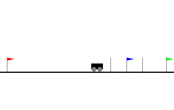
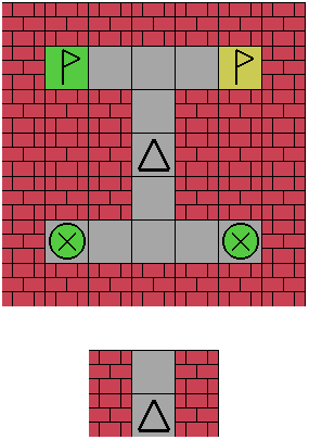
In the CarFlag domain, the agent must go to the green flag (can be on any side). If it goes to the red flag, it is penalized (-1). If it goes to the blue flag, the agent learns the direction of the green flag (reward of +1).
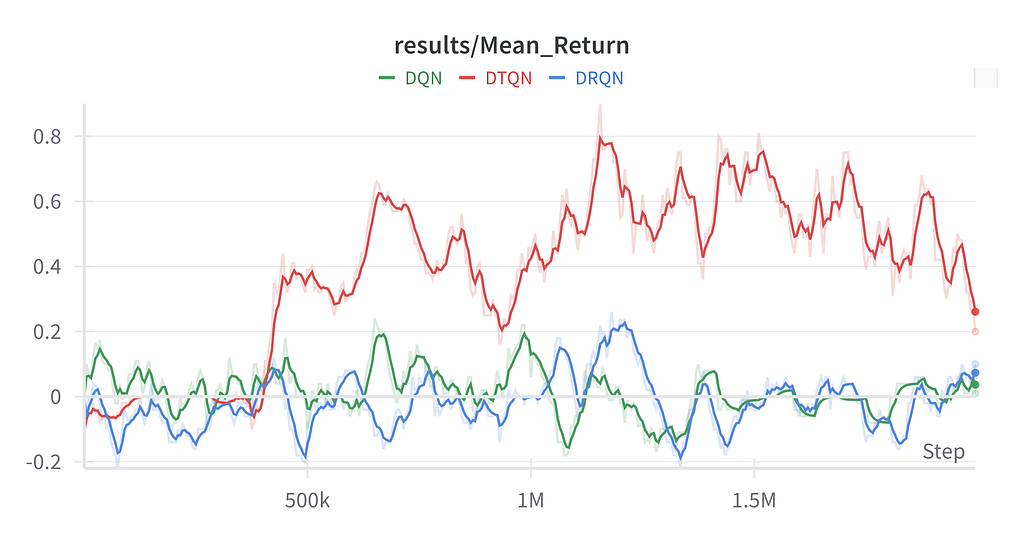
Initially, we said that the goal of an agent in reinforcement learning is to maximize its final reward. From the image below (learning curves), we can see that in the CarFlag environment, DTQN provided the best return as it was allowed to take steps in the environment and train.
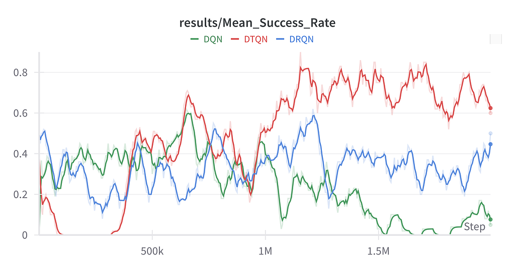
We also have data on how successful the agent was with every algorithm.
Discussion of Results
The paper shows results of DTQN outperforming (or comparable performance to) DRQN in most environments in which it was tested. The ablation results only show a significant improvement when Intermediate Q-values are trained on (i.e. train on the Q-values generated for each timestep in the observation history). The other ablations do not seem to offer a significant performance improvement. One interesting thing to note from the results obtained by the authors is that they can now visualize the most important parts of an agent's history of observations for decision-making. I find this quite fascinating for explainable AI in an RL context.
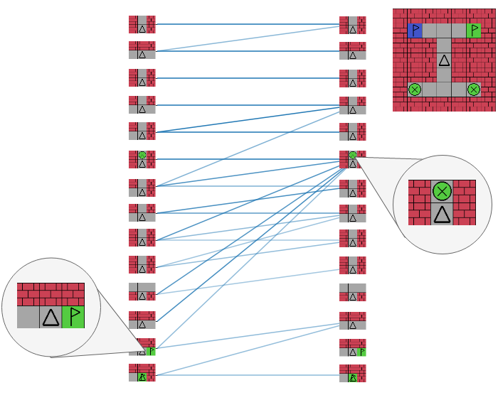
The authors provided a great example of the observation history in the Gridverse domain, with high attention weights highlighted in the image.
I would like to note, however, that the environments being tested in the paper were rather small. Both state and action spaces were limited in the tested domain. A larger domain is necessary to see how well this method can compare to DRQN and traditional POMDP solvers.
<hr><p>Deep Transformer Q Networks — A paper analysis was originally published in Toward Humanoids on Medium, where people are continuing the conversation by highlighting and responding to this story.</p>